# Run shiny app
hsi_tools_core <- HSItools::run_core()2 Shiny app
Our shiny app allows quick choice of data, settings, regions of interest (ROI), and depth calibration. Here, we walk through the entire app, screen by screen.
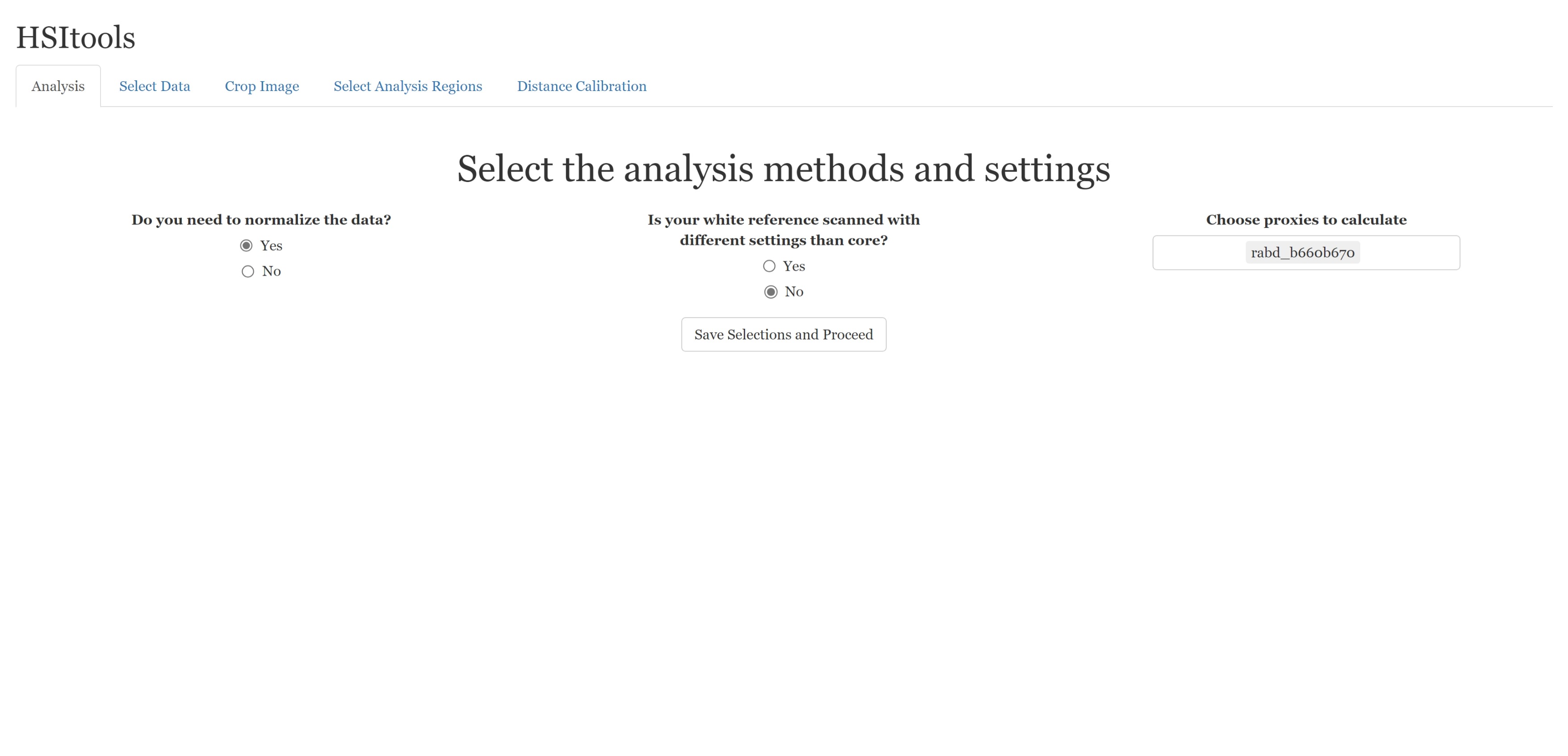
2.1 Screen 1: Initial settings
On this screen, you have to make an initial choice. First, you need to decide whether to normalize data. If you have a reflectance file from other software, like Lumo®, you probably do not need to normalize the file from the beginning—this is one of the most time-consuming processes.
Suppose you decide that you need to normalize your data. In that case, you can select other integration times for your white and dark references if you scanned your target with different settings for target and references. This can happen if you were worried about white reference overexposure, whereas your target was very dark. Finally, you can select some proposed HSI indices from the defaults.
Indices
At the moment, selecting indices will not do anything in particular.
Run the Shiny app.
2.2 Screen 2: Data choice
This screen lets you decide whether to use your data or the provided example.
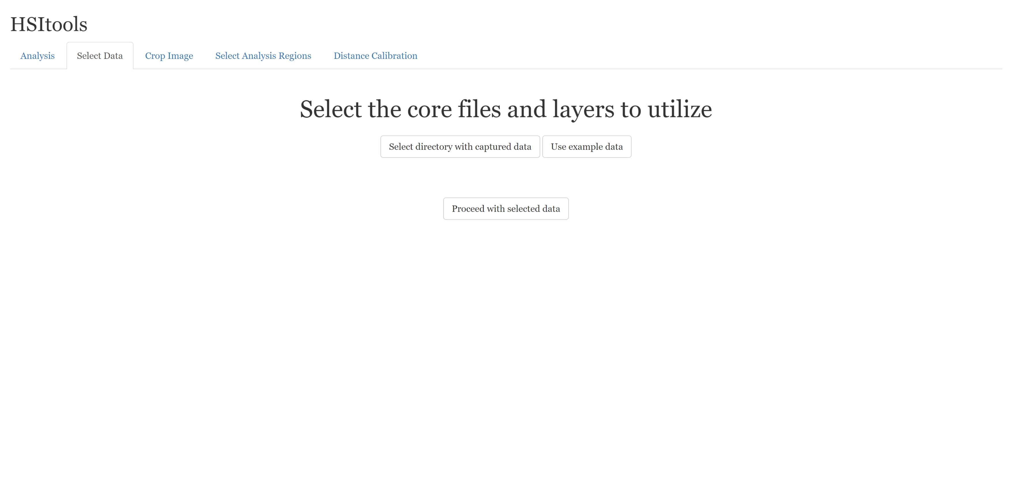
You can select your data from your drive once you use it. Be sure that it is stored on the SSD drive. Here, it is essential that you do not go all the way to the capture folder but rather point to the root directory of your selected scan.
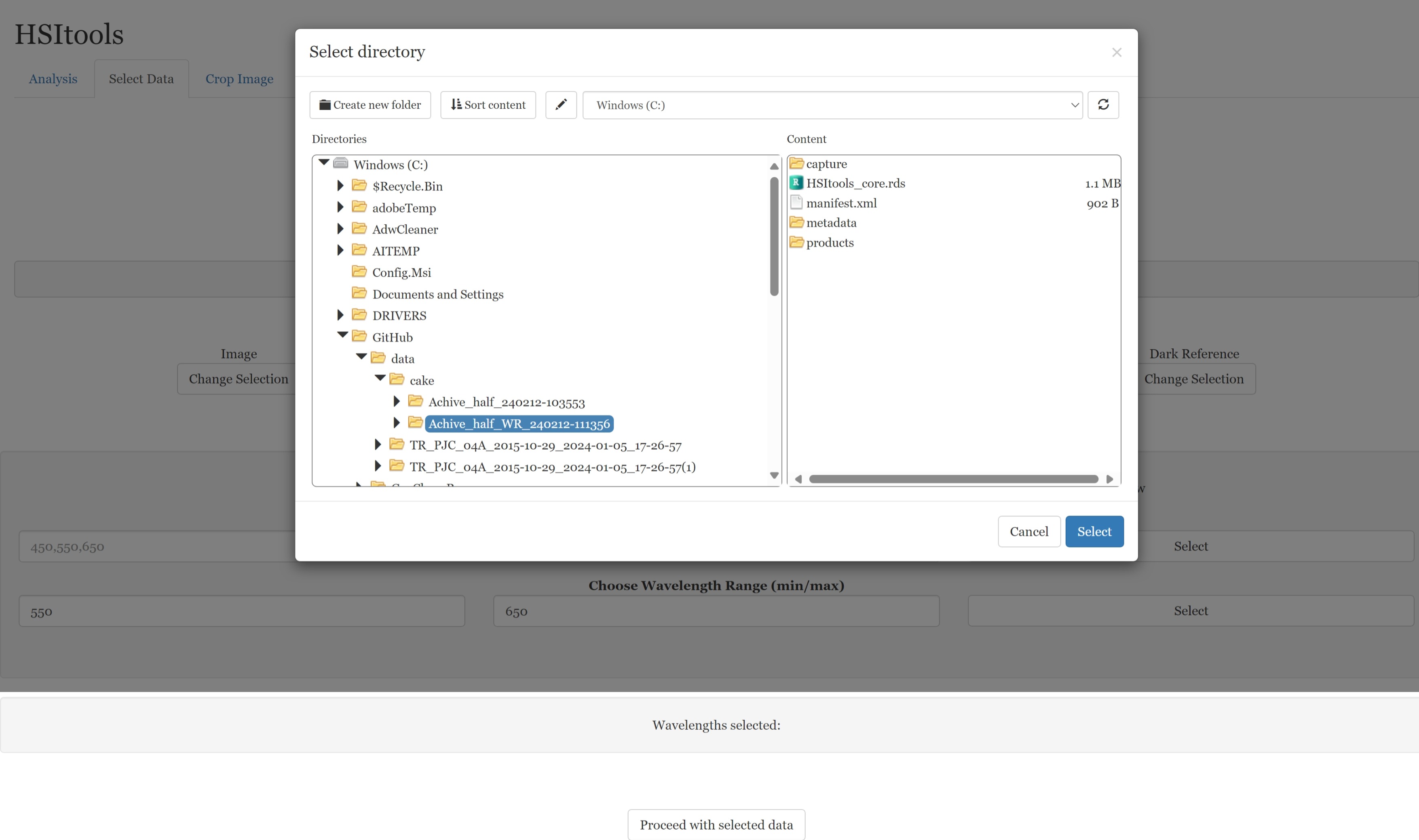
Once you’ve selected data, you can choose the raster files, bypassing our heuristics and default search patterns in the “capture” directory. At this point, you’ll also get some basic information on your raster dimensions.
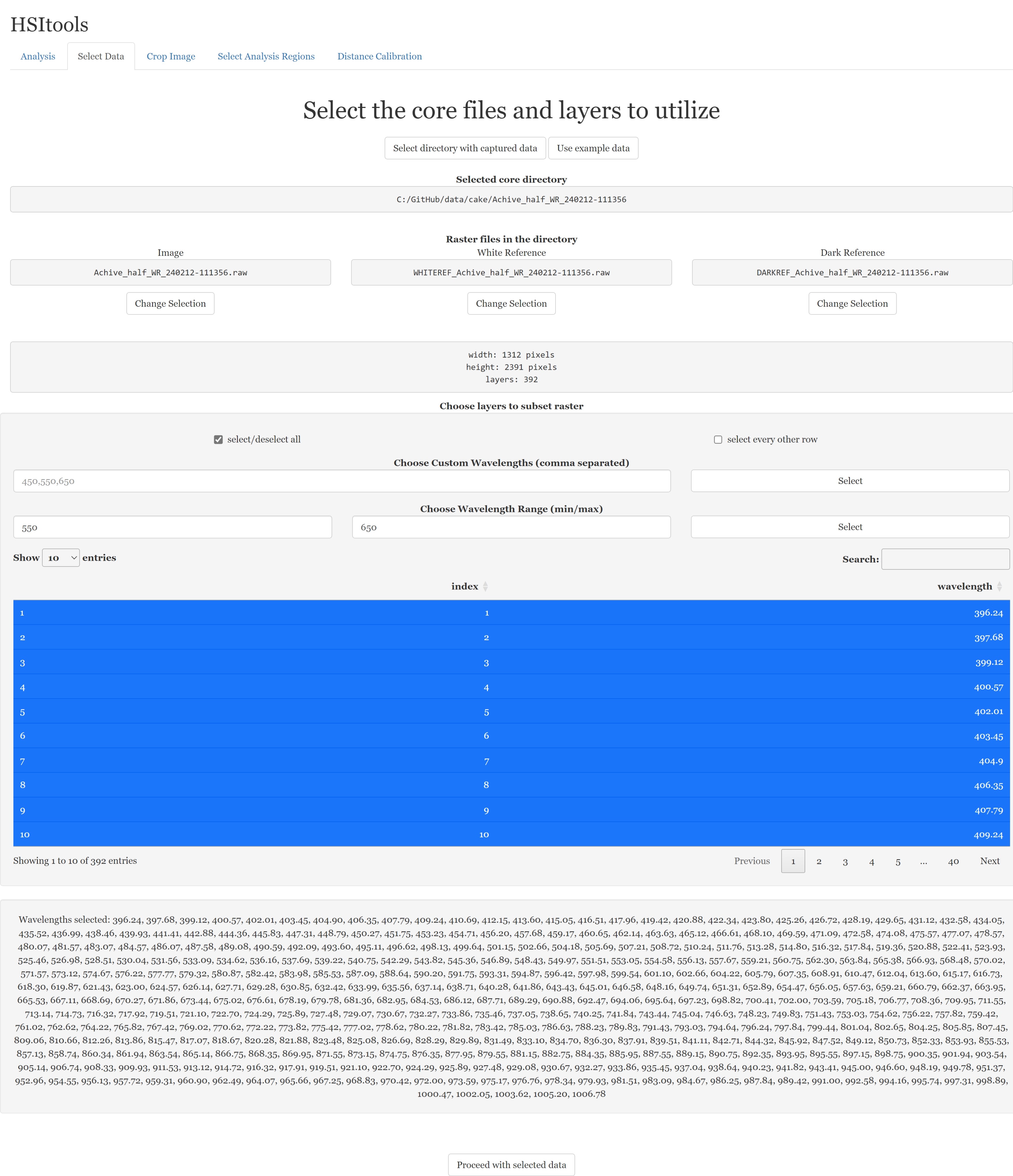
Once you’re happy with your data choice, select layers (bands) to work with.

If you’re happy with your choices, scroll down and proceed.

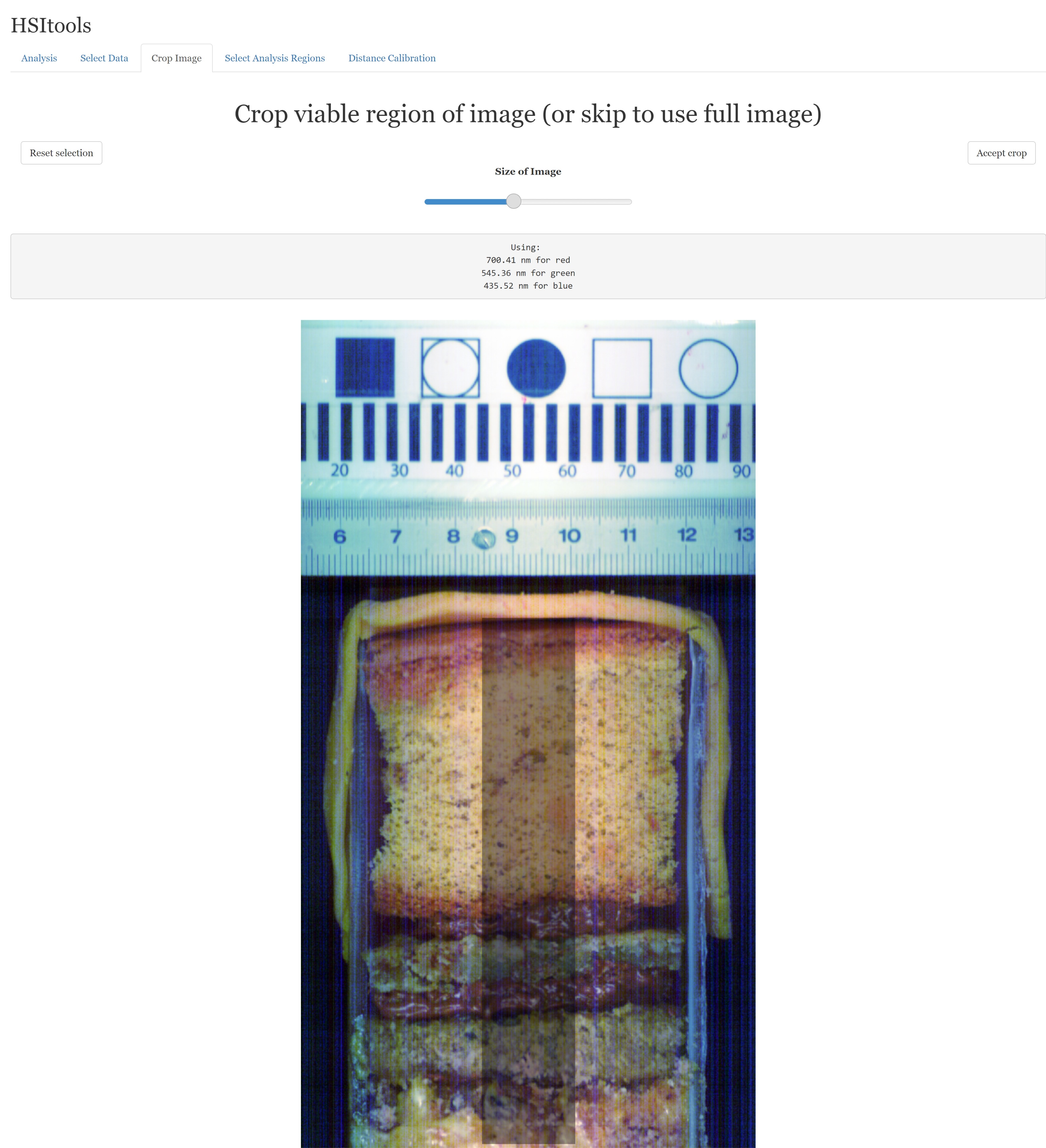
2.3 Screen 3: Cropping
Here, you can crop your data (raster). You can see the bounding box of the cropped data. If it helps, you can change the size of the image. Leave a pixel or two on the edges; if pushed to the extremes, it can mess up the cropping. Once you’re happy, accept the crop and proceed.
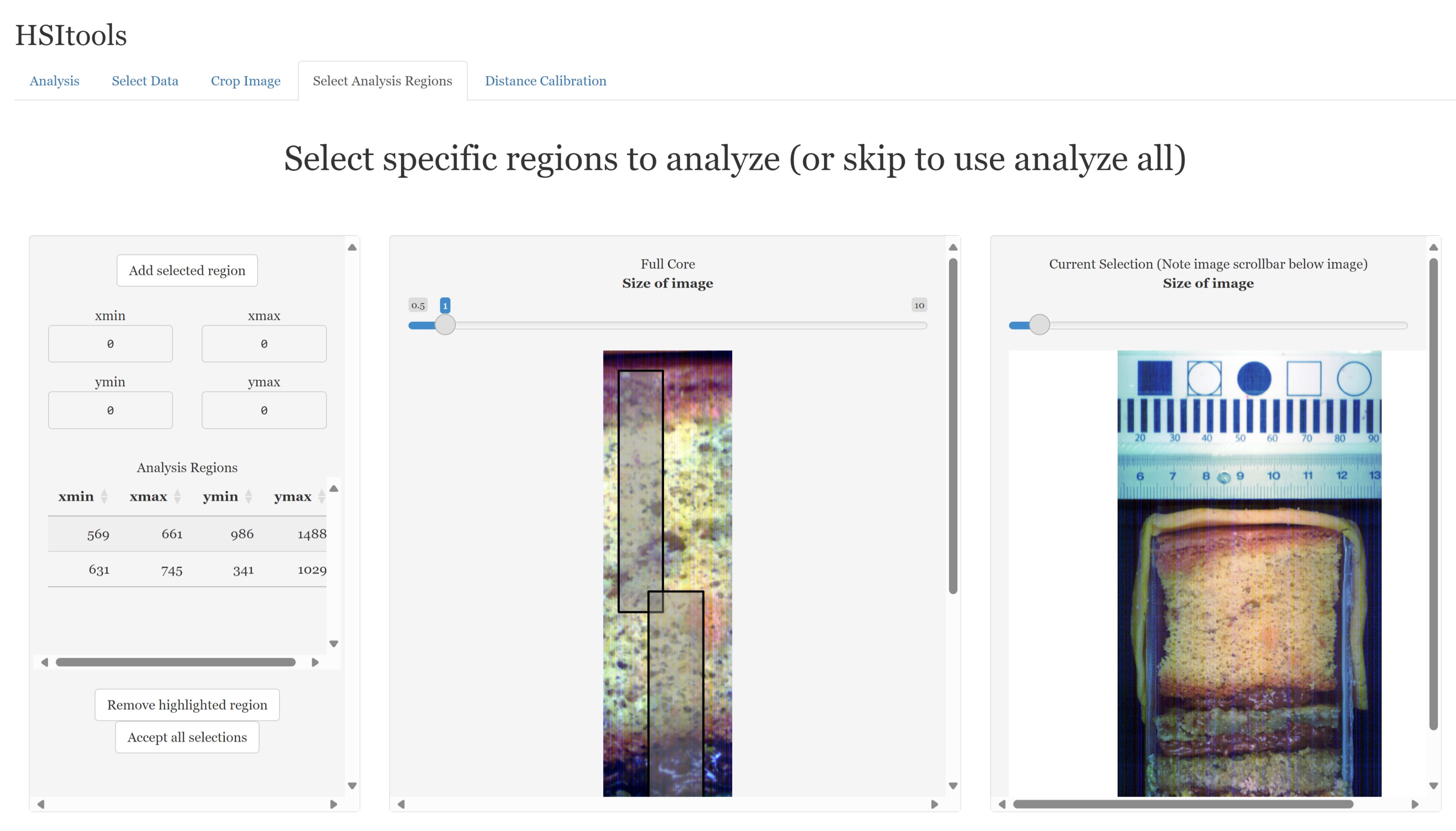
2.4 Screen 4: ROI selection
Here, you can select the regions of interest (ROI) you want to work over rather than calculating the entire data. These ROIs are strictly rectangular, so we prefer the GIS approach with masking. Please select the region, then add it using the button. Repeat for as many regions as you need. On the right, you have a zoom of your selection. Once you’re happy with your ROIs, accept and proceed.
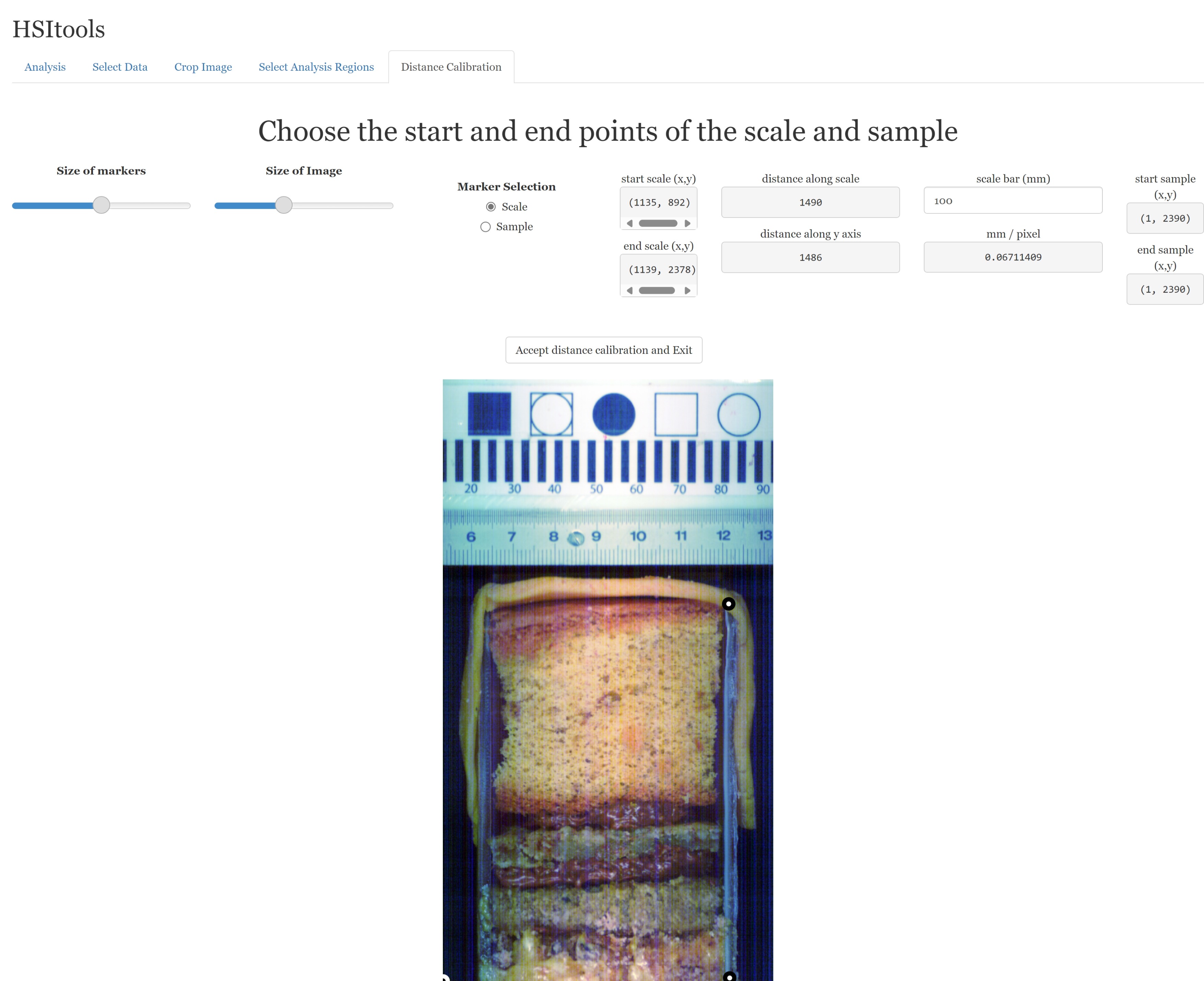
2.5 Screen 5: Calibration
Finally, it is time to calibrate your data.
First, we calibrate the distance. Simply put, we want to know the actual distance in one pixel. For this, we use the tape measure and put the two markers. Then, we read the depth from the tape—the further the distance between the points, the better. We use only 20 mm, so it fits on the screen. Our equation takes into account both the distance and angle.
Finally, we put in the second set of markers, which tracks the actual beginning and end of the scanned sample—the true-zero is essential here.
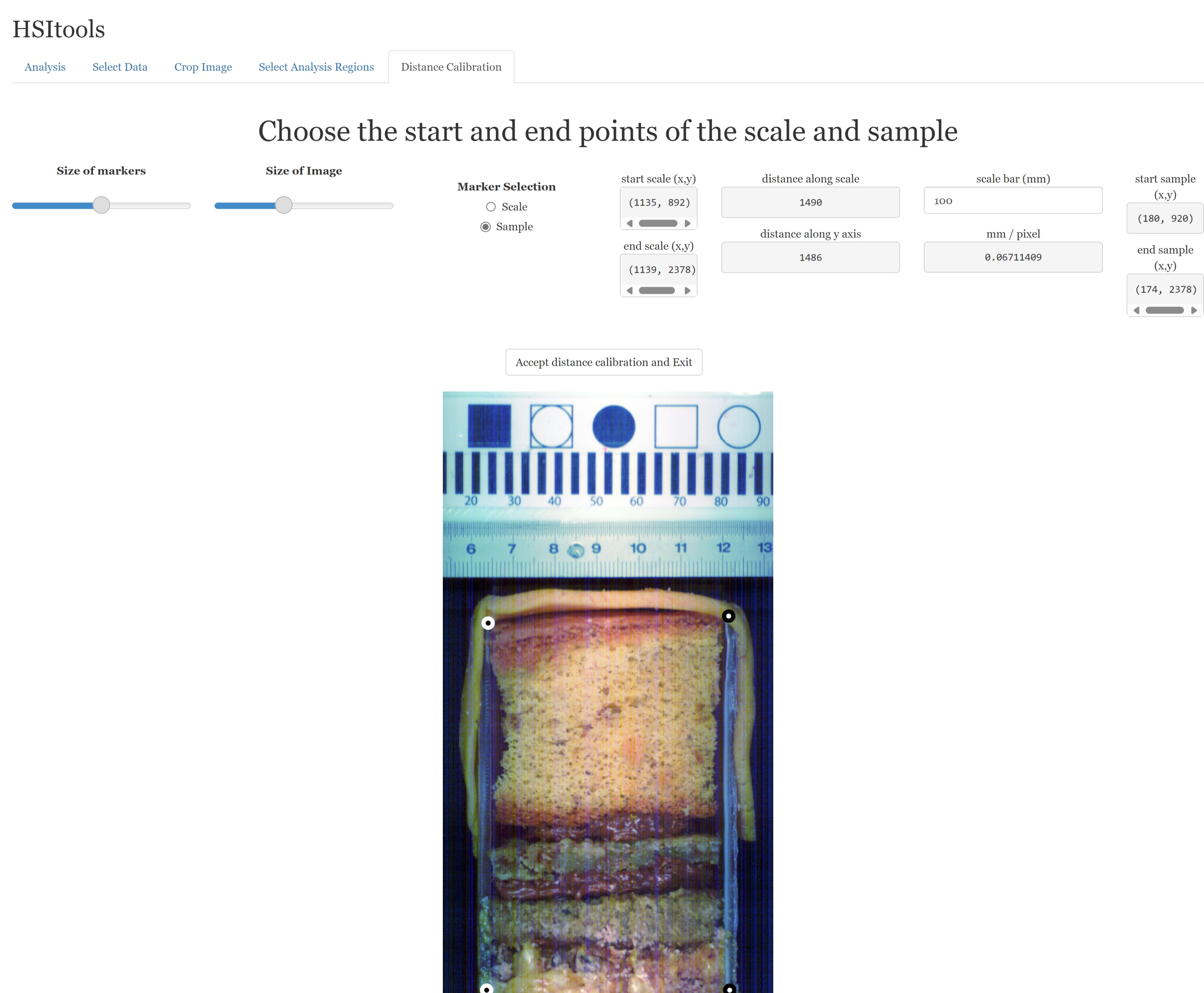
Once you select both sets of markers, accept and exit the app.