# Preview RGB
p_rgb <- reflectance |>
  # Plot
1  plot_raster_rgb(
2    calibration = pixel_to_distance(hsi_tools_core)
  )

# Print
p_rgb- 1
- Function to plot RGB.
- 2
- Call to HSItools core output of the Shiny app storing the depth calibration.
Preview RGB with the scale. In all of the following functions, you can call the extent argument.
# Preview RGB
p_rgb <- reflectance |>
# Plot
1 plot_raster_rgb(
2 calibration = pixel_to_distance(hsi_tools_core)
)
# Print
p_rgb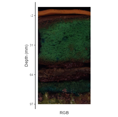
For example, we can plot the spatial map of RABD660:670max.
# Plot RABD
p_rabd <- rabd_max |>
1  plot_raster_proxy(
2    hsi_index = names(rabd),
3    calibration = pixel_to_distance(hsi_tools_core),
4    palette = "viridis",
  )

# Print
p_rabd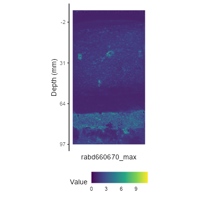
We can extract profile of the selected index using one of the predefined ROIs. We use the small, green ROI in the middle.
# Plot series
p_rabd_series <- rabd |>
  # Plot
1  HSItools::plot_profile_spectral_series(
2    hsi_index = names(rabd),
3    calibration = pixel_to_distance(hsi_tools_core),

# Print
p_rabd_series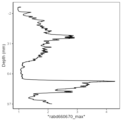
We can display it side by side using the magic of {patchwork}.
# Plot using {patchwork}
p_rgb + p_rabd + p_rabd_series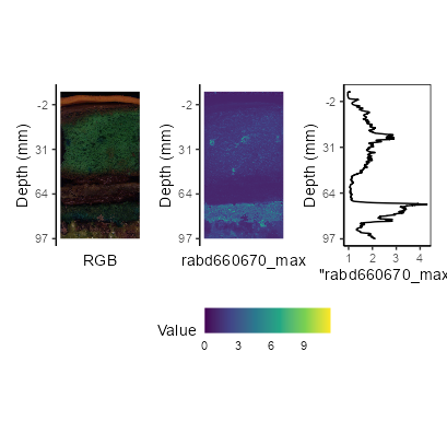
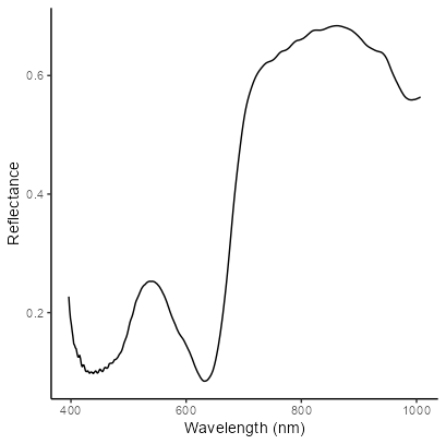
Finally, you might be interested in plotting the average spectrum from the selected area. We’ll use the uppermost “sample” from the ROI preview.
# Plot reflectance profile
p_sample <- reflectance |>
1  plot_profile_spectral_profile()

# Print
p_sample